Introduction
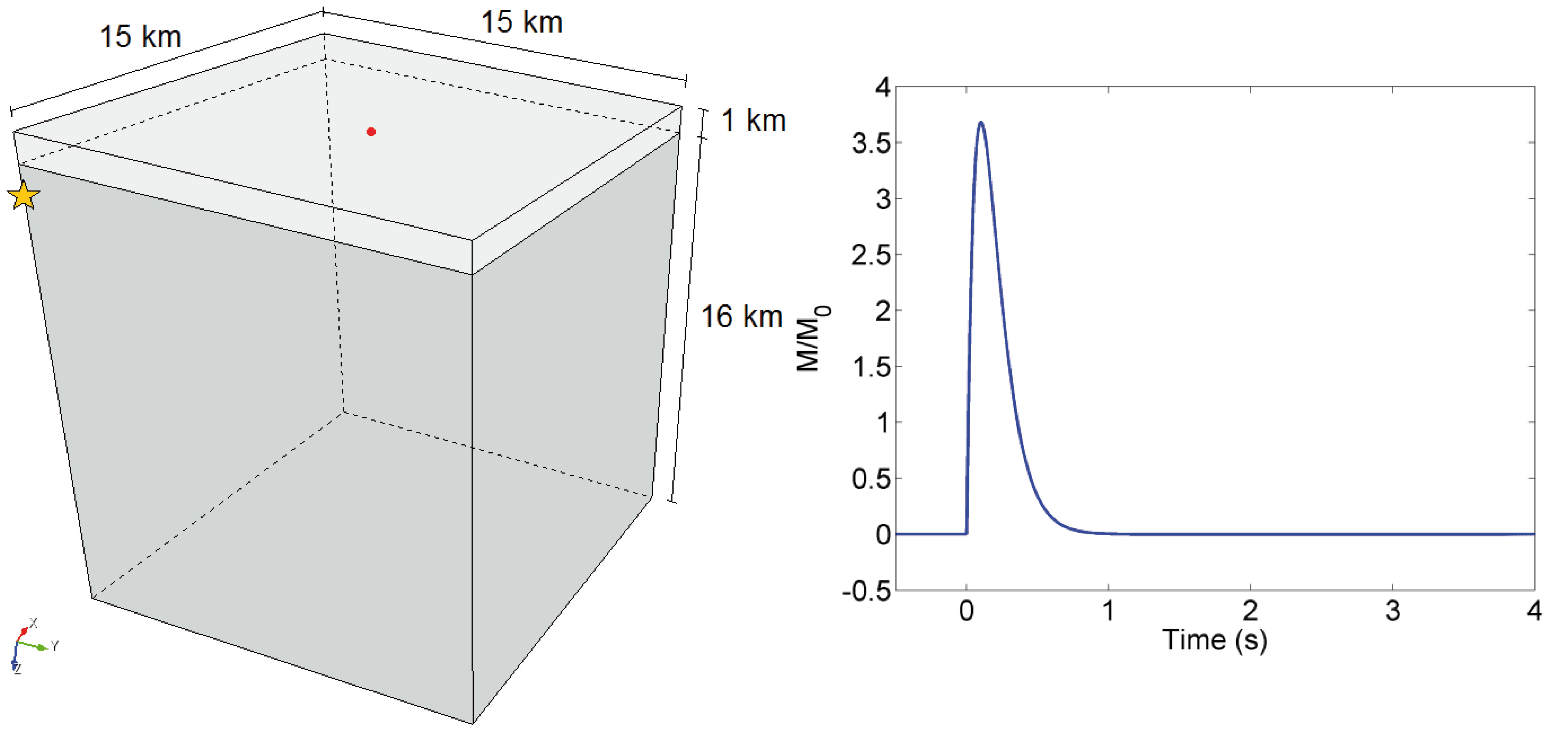
Left hand side: layer over halfspace Benchmark test, only one of the four symmetric quadrants is shown, the source (yellow star) is located at 2 km depth and different colors mean different mechanical characteristics; in red the receiver considered. Right hand side: moment rate function for the validation-test.
Problem set up
Further details on the problem setting as well as on the source time function can be found in Day et al. (2001), together with the expression of the semi-analytic solution. In this case, two different models were considered and implemented in SPEED, the first one relying on a conforming spectral element discretization and the second one by using the DGSE approach described earlier.
The characteristics of the numerical models and the main parameters of the analysis are listed below.
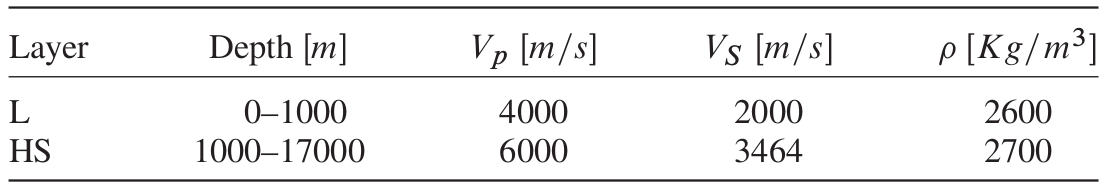
Dynamic and mechanical parameters for the layer (L) and the halfspace (HS) of the layer over halfspace test.
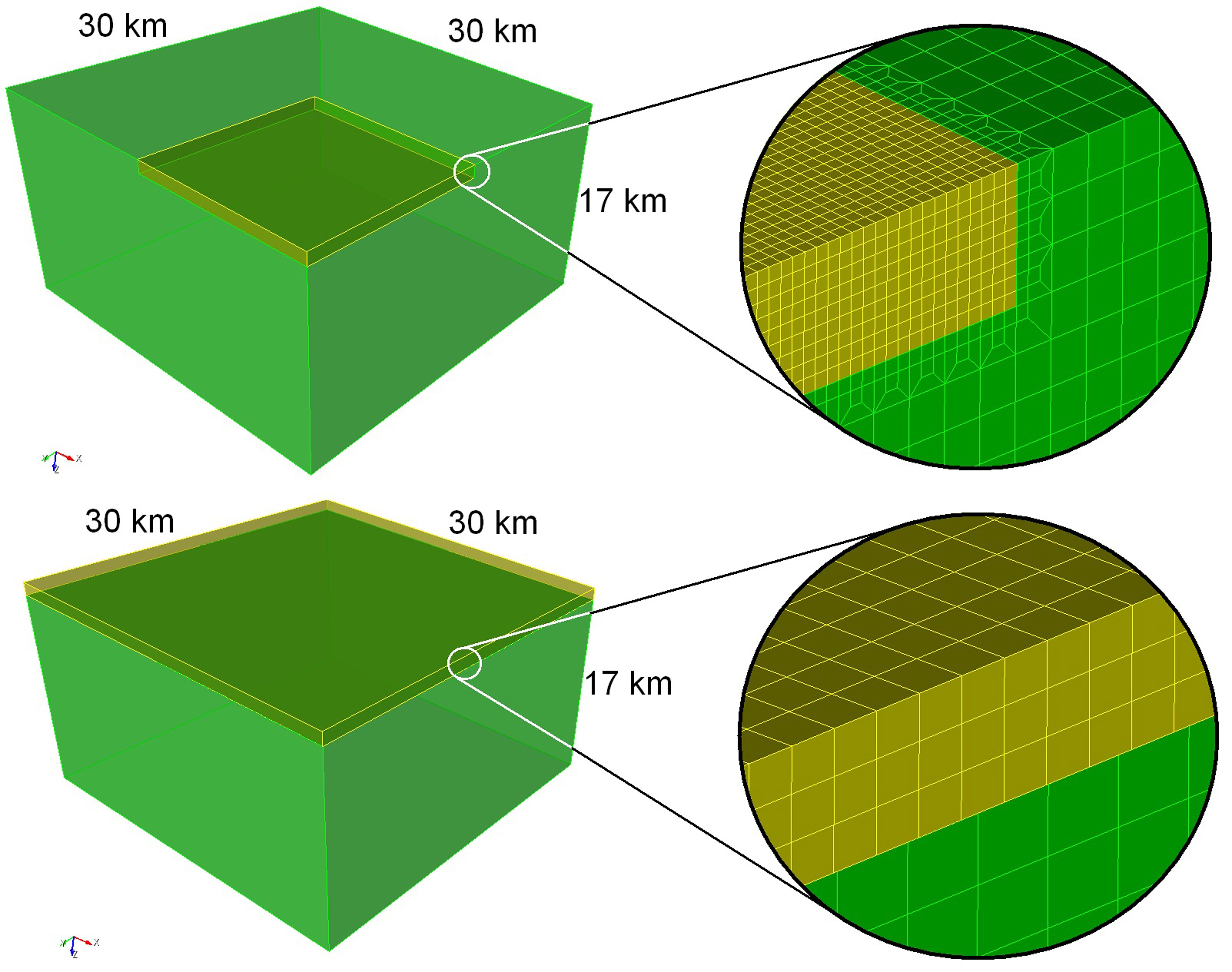
Layer over halfspace conforming model, having size of 30 x 30 x 17 km: (top) conforming mesh with 814.833 hexahedral elements, varying from size of 100 m, in the first quadrant, to 300 m in the remaining part of the domain; (bottom) non-conforming model with 70.228 hexahedral elements, having size of around 400 m in the upper layer (1 km thickness) and size of around 650 m in the lower layer (16 km thickness).
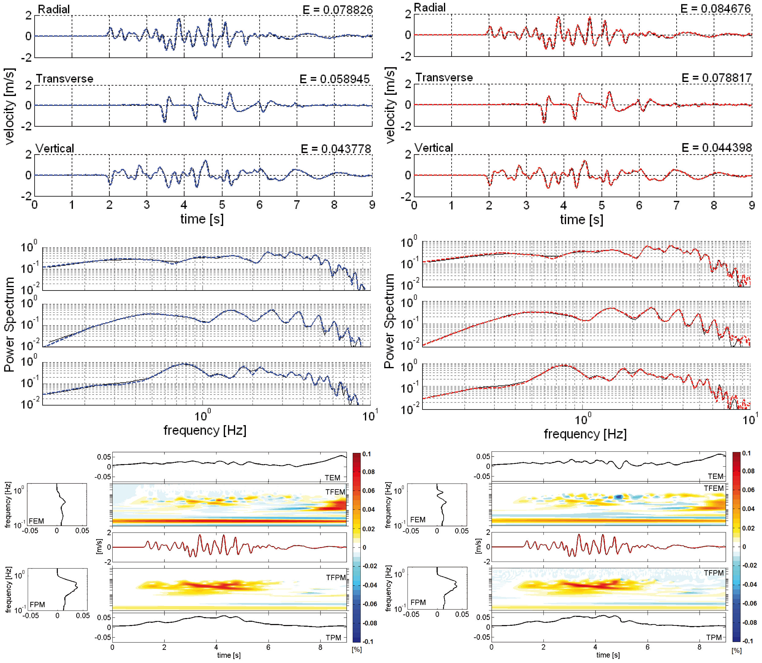
Velocity field recorded at (6, 8, 0) km. Comparison in the time and frequency domain between the semi-analytic solution (black line) and the numerical one (colored line). Relative misfit computed for the signal along x axis (FEM , frequency-dependent envelope misfit; TEM , time-dependent envelope misfit; TFEM, time-frequency envelope misfit; FPM, frequency-dependent phase misfit; TPM, time-dependent phase misfit; TFPM, Time-frequency phase misfit. Percentage values.). Left hand side, conforming model; right hand side, non-conforming model.
Numerical Results
We report the velocity wave field recorded at point (6, 8, 0) km on the top layer along with the reference solution. In each plot, we also report the relative seismogram misfit, see Kristekova et al. (2006).
The maximum relative misfit with respect to the reference solution is less than 1% for the conforming model and around 2% for the non-conforming one. It is important to underline that the non-conforming model has a sensibly lower number of elements, nonetheless the accuracy of the solution is preserved. These results are promising, especially compared with those available in literature (see, e.g., Käser et al. 2007, Stupazzini et al. 2009).
References
Day SM, Bradley CR. Memory-efficient simulation of anelastic wave propagation. Bulletin of the Seismological Society of America 2001; 91(3):520–531.
Käser, M., M. Dumbser, J. De la Puente, and H. Igel (2007). An arbitrary high order discontinuous Galerkin method for elastic waves on unstructured meshes iii: viscoelasti attenuation, Geophys. J. Int. 168, 224–242.
Kristekova M, Kristek J, Moczo P, Day SM. Misfit criteria for quantitative comparison of seismograms. Bulletin of the Seismological Society of America 2006; 96(5):1836–1850.
Stupazzini M., R. Paolucci R. and H. Igel (2009), Near-fault earthquake ground motion simulation in the Grenoble Valley by a high-performance spectral element code. Bull. Seismol. Soc. Am., 99(1), 286-301.