I. Mazzieri, L. Melas, C. Smerzini, M. Stupazzini (2018). The role of near-field ground motion on seismic risk assessment in large urban areas. In Proceedings of the 16th European Conference on Earthquake Engineering, 16 ECEE 2018, Paper No 1024.
Why the Beijing area
Situated on a sedimentary basin, with its more than 20 million inhabitants, Beijing is one of the many megacities around the world highly exposed to the seismic threat. As a matter of fact, in the past thousand years, many destructive earthquakes have occurred in the area around Beijing, with magnitude varying from Mw 6 to Mw 6.5 (Gao et al. 2015 and references therein). Combining physics-based fault rupture scenarios with up-to-date fragility curves, seismic damage scenarios have been produced for the urban area of Beijing, with reference to the class of high-rise buildings, which represent an important proportion of assets at risk.
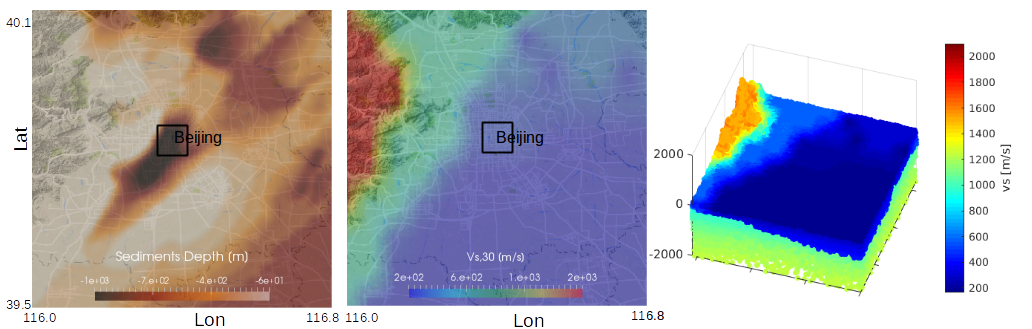
Figure 1. Sediment thickness (left), VS30 model (center) and VS(z) model (right) for the first layer 0-2 km.
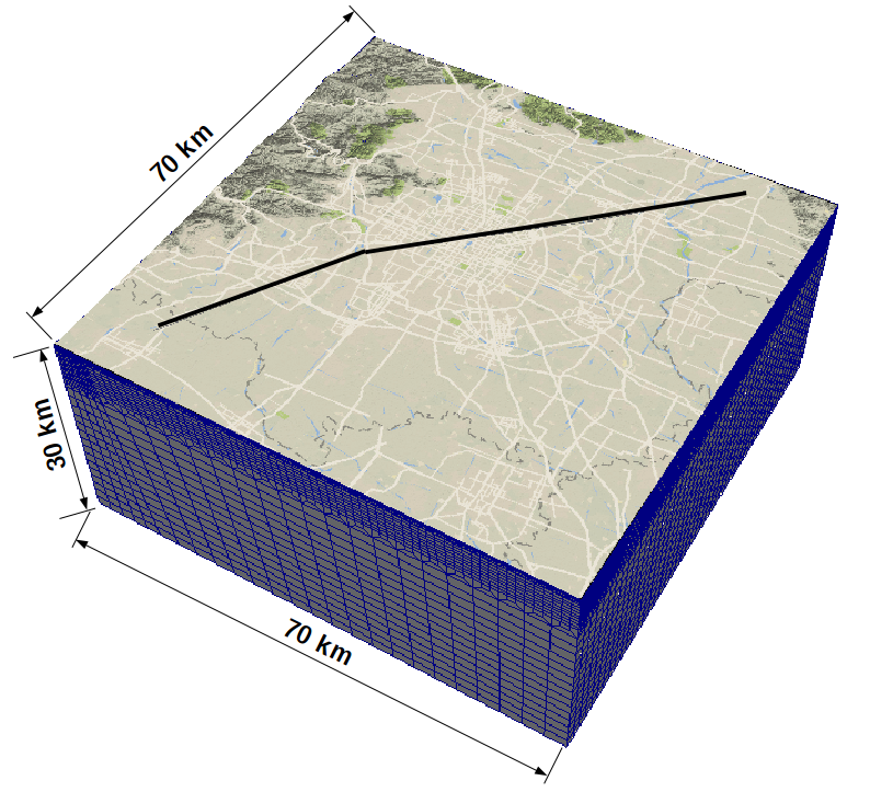
Figure 2. 3D computational model for the Beijing area. Black segments represent the trace of the considered Shunyi-Qianmen-Liangxiang fault.
Numerical model
The 3D numerical model for the Beijing area encompasses the following features: i) the topography model; ii) a kinematic model for the seismic fault rupture; iii) the 3D basin model, defined from the depth of basement of sedimentary deposits and shear wave velocity profiles, cf. Figure 1.
The seismic fault considered consists of the Shunyi-Qianmen-Liangxiang (SQL) fault, lying just through the downtown of Beijing (see superimposed line in Figure 2). The source is a quasi-vertical segmented fault (with dip angle of about 80°), consisting approximately of three main segments with different strike angles. The total length of the fault is about 90 km, considered therefore capable of producing up to magnitude 7.3 events.
The computational model was then set up by combining all information above and extends over an area of 70 km x 70 km down to 30 km depth, as illustrated in Figure 2. The conforming mesh has a size varying from a minimum of 150 m, on the top surface, up to 600 m at 4 km depth and reaching 1800 m in the underlying layers. The model consists of 859,677 hexahedral elements, resulting in approximately 160 million degrees of freedom, using a fourth order polynomial approximation degree.
Summary of simulated ground shaking scenarios
A total of 30 scenarios were simulated by varying the magnitude, from 6.5 up to 7.3, the kinematic slip distribution, the hypocenter location and the location of the rupture area.
The numerical results obtained by SPEED are substantially in agreement with the GMPE proposed by Cauzzi et al. 2015. However, synthetic scenarios produce higher PGVs in the proximity of the fault rupture. This may have a great impact on seismic hazard estimates, as standard GMPEs cannot account for such effects. In Figure 3 we report some snapshots of the peak ground velocity wave field for a target scenario with magnitude Mw 7.3. It is possible to notice that the wave field propagates in the direction south-west to north-east and that higher values of PGV are obtained closed to the projection of the fault rupture on the surface, as to be expected.
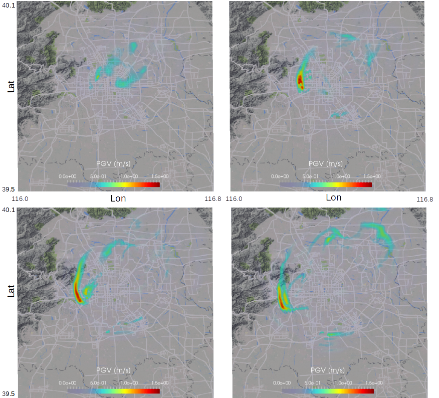
Figure 3. Snapshots of the PGV obtained for a scenario with Mw 7.3. Top-left: t = 8 s, top-right: t = 9 s, bottom-left: t = 10 s, bottom-right: t = 11 s.
Results of the analysis
Due to the fact that we are interested in investigating approximately 100 meters high-rise buildings, we decided to use the Spectra Displacement at 3 second as ground motion proxy. Out of that and adopting the fragility curves by Wu et al. 2013, we calculated the probability of different building performance levels and therefore in ultimate analysis the overall damage.
Figure 4 shows the results obtained out of the four scenarios in terms of the probability of exceedance of the different Damage States. The black dots show the mean probability given a certain distance and the bars represent the standard deviation around the mean. It is worth to note the large dispersion around the mean value and once again the extremely rapid decrease of the probabilities associated to different damage state with respect to the Rrupt.
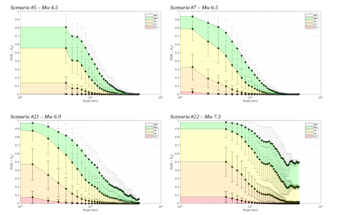
Figure 4. Normalized probability for all damage states (DS) versus the closest distance to the fault rupture (Rrupt). The different colors denote the P(DS=DS) for each VRG point (white: no damages – ND; green: very light damages, normal operation – NO; yellow: light damages, immediate operation – IO; orange: moderate damages, life security – LS; red: severe damages, collapse prevention – CP), while filled black dots represent the mean of P(DS= DS) at a given distance and the black bars represent the corresponding standard deviation.
References
Cauzzi C, Faccioli E, Vanini M, Bianchini A (2015): Update predictive equations for broadband (0.01 to 10 s) horizontal response spectra and peak ground motions, based on a global dataset of digital acceleration records, Bulletin of Earthquake Engineering, 13/6, 1578-612.
Gao M, Yu Y, Zhang X, Wu J (2015): Three-dimensional finite-difference modeling of ground motion in Beijing from a Mw 7 scenario earthquake. In Proceedings of the 13th World Conference on Earthquake Engineering, Paper No 581.
Wu F, Wang M, Yang X Y (2013): Building seismic vulnerability study for China high rises. In Advances in Civil and Industrial Engineering. Applied Mechanics and Material, vol. 353: pp 2301-2304.